
Global climate models (GCMs) provide the best estimates of global change to our climate to the end of the 21st century. Using more global climate models in a climate modelling study gives a better idea of the range of possible future climate conditions, allowing us to be more confident in the projected change in the Earth’s climate. The Intergovernmental Panel on Climate Change (IPCC) considered output from 23 global climate models when compiling its Fourth Assessment Report. Climate Futures for Tasmania used the same multi-model approach. However due to the modest scale of the project relative to the IPCC AR4, we used six GCMs. As the ability to accurately simulate present climate is a useful indicator of how well a model can simulate the future climate, we chose the six models for their ability to reproduce present day rainfall means and variability over Australia.
Generally, climate information from global climate models has a resolution of 200 km to 300 km. This means that the Earth’s surface is divided into grid cells that are 200 km to 300 km along each side. At this resolution, a single state of Australia may be represented by only a few grid cells. In each grid cell, climate variables such as temperature and rainfall, and even the topography, have just a single value. This means global climate models do not allow us to understand the regional detail of climate change at local scales, for example they can not distinguish between valleys, coastlines and mountains. For this level of detail, we downscale information from global climate models using an advanced dynamical model.
It is very likely that rising greenhouse gases, along with aerosol emissions, stratospheric ozone depletion and other human influences, are responsible for much of the recent global climate change. The extent of future man-made climate change is dependent on the amount of greenhouse gases and other emissions that are released. The most commonly used and accepted set of emissions scenarios comes from the Intergovernmental Panel on Climate Change (IPCC), who outlined the scenarios in their 2001 Special Report on Emissions Scenarios (SRES). These scenarios, commonly referred to as SRES scenarios, are divided into six ‘families’ – A1FI, A2, A1B, B2, A1T and B1 – and are based on estimated future technological and societal (such as population growth) changes.
Climate Futures for Tasmania used a high emissions scenario (A2) and a low emissions scenario (B1). Using a high and a low emissions scenario provides a reasonable upper and lower range of climate change projections. It is worth noting that these emissions scenarios do not diverge significantly until the middle of the 21st century and thus the change in global mean near‑surface temperature is roughly the same across all emissions scenarios up until the middle of the century. Consequently, the choice of SRES emissions scenario does not become important until the latter half of the century.
There are two established methods for downscaling global climate model information to a finer scale suitable for regional studies: dynamical downscaling and statistical downscaling. Dynamical downscaling uses output from a ‘host’ global climate model as input into either a limited-area climate model or a stretched grid global climate model. Limited area climate models operate over a small part of the globe. Stretched grid global climate models operate over the entire globe, but focus on one small area in particular.
Regional climate models use the same physics as global climate models, and can be just as complex; however, because a regional model focuses on a small area, it provides more detail over that area than a global model, and is much more efficient and economical to
run.
Statistical downscaling relates patterns and changes in large scale climate to the local climate. These statistical relationships are derived from historical observations. Once established, the relationships are applied to global climate model projections to produce
fine-scale projections of local climate. Statistical downscaling is usually much less complex, and requires much less computing power, than dynamical downscaling. Statistical and dynamical downscaling produce similar results for present-day climate, but
can differ when examining future climate projections. Statistical downscaling applies historically observed links between large-scale climate variables (from the global climate model) and local climate to a future climate. This is often considered a limitation of statistical downscaling, as these relationships may change in a warmer world. Dynamical downscaling models are complex enough to allow relationships between large-scale climate and local climate to change under future climate according to our understanding of atmospheric processes. A second limitation of projecting a changing climate using statistical downscaling is that the observations being used for the downscaling must span the range of projected future climate responses. In practice, this requires long, reliable observations of both the large and fine-scale climate. Such observational datasets are often not available. Dynamical models rely on our understanding of physical processes in the atmosphere, not only observations of climate.
Dynamical models are complex enough to simulate climate and climate changes at all scales, from global to regional, in a coherent manner. Using dynamical downscaling allows us to demonstrate changes in the local climate of Tasmania, such as changes to the timing, frequency and intensity of weather events – changes that are difficult to detect using statistical downscaling. Dynamical downscaling also maintains the relationships between different climate variables. For example, ‘rainy days’ will be ‘cloudy’ and ‘cool’, or when a ‘cold front’ passes over Tasmania the ‘temperature’ drops. This allows us to assess complex changes, for example changes to agricultural production, that involve the interaction of many climate variables (for example, the incidence of frost and available water). The main constraint of dynamical downscaling is the technical complexity and computational cost. Because of the many benefits of dynamical downscaling, Climate Futures for Tasmania made the technical and financial commitment to use dynamical downscaling
Downscaling can lead to a different story: The global climate model (top image) shows that summer rainfall is projected to decrease in the future. As we downscale from the global climate model (middle and bottom image) projections show an increase in summer rainfall on the east coast of Tasmania. This different projection is due to the improved ability of the downscaled simulations to model drivers of Tasmanian rainfall.
Tasmania is roughly 350 km by 300 km, the size of a few global climate model grid cells. After carefully weighing up the costs and benefits involved with downscaling to different grid-scales, Climate Futures for Tasmania decided on a final resolution of 0.1 degrees . This corresponds to a grid where each individual cell has side lengths of approximately 10 km. To achieve this resolution we undertook a two-stage dynamical downscaling process using CSIRO’s Conformal Cubic Atmospheric Model (CCAM). The two-stage process used sea surface temperature from the six selected global climate models (for each of the two SRES emissions scenarios) to create intermediate resolution simulations with a resolution of 0.5 degrees (around 60 km) over Australia.
Before we use the modelling output from the global climate models, we bias-adjust the sea surface temperature to bring the modelling output in line with the observed temperatures. These intermediate-resolution simulations are used as input for the simulations with a high-resolution over Tasmania (0.1 degrees or 10 km). We also produce a simulation with very high resolution over Tasmania (0.05-degrees) using the A2 emissions scenario and CSIRO-Mk3.5 as the host global climate model. The temperature of the sea surface is a major factor in driving global climate systems (such as the monsoons, El Niño or the Roaring Forties), that in turn influence the local climate and weather conditions. Sea surface temperature (and sea-ice concentration in the polar regions) is the only information from the global climate model we use in the downscaling process. By only using information from the ocean surface, we allow the regional climate simulations to create their own pressure, wind, temperature and rainfall patterns in the atmosphere. These patterns occur in response to such local effects as topography. Using the sea surface temperatures from the host global climate model ensures the large-scale climate is the same as the global model.
Running a climate simulation to generate a projection of future climate is just like running an experiment. The more often you repeat an experiment and get a similar answer, the more trustworthy the results. To test whether our projections of future climate are realistic, we run many simulations and study the similarities (and differences) in the results. Just like cars, there are many types of global climate models. Some models are produced in the UK (UKMO‑HadCM3), some in the US (GFDL-CM2.0 and GFDL-CM2.1),
Japan (MIROC3.2(medres)), Germany (ECHAM5/MPI-OM), Australia (CSIRO-Mk3.5) and several other nations. Using six global climate models allows us to repeat the experiment six times. Where the simulations agree we have increased confidence in our projections. The differences between the simulations allow us to estimate the uncertainty in our projections.
Global climate models do not know anything about the current climate aside from the composition of the atmosphere and radiation from the sun. They generate a completely simulated climate, that is, no observations of the current weather or climate have been used to steer them. The downscaled simulations only know the bias-adjusted sea surface temperature from the global climate models. They are not told about past weather and thus, there is no direct link between the simulations and the observed records. This means that we can test the skill of our model in simulating a realistic climate by comparing the simulations representing the recent past with observations in the same period. The dynamically downscaled simulations have a high level of skill in reproducing the recent climate of Tasmania across a range of climate variables.
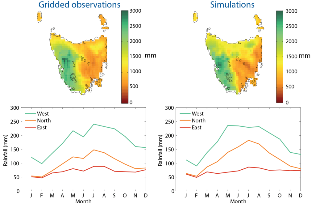
Figure: Comparing observations and simulations
Comparing our simulations to observations (the Bureau of Meteorology’s AWAP* dataset) for the period 1961-2007, shows that the central estimate (the average of the six simulations) of statewide daily maximum temperature is within 0.1°C of the observed
value of 10.4 °C. The simulated average annual rainfall of 1385 mm is very close to the observed value of 1390 mm. The maps of Tasmania (at left) show that the simulations reproduce the spatial pattern of rainfall over the state. For example, high rainfall in the south-west and a drier east coast and Derwent Valley.
Similarly, the dynamically downscaled models reproduce the different seasonality in climate variables (for example, rainfall) in different regions of Tasmania. The graphs show the monthly rainfall in three regions of Tasmania. The simulations reproduce the wet winters and drier summers on the west coast and the consistently low rainfall throughout the year on the east coast. The downscaled simulations have reproduced the spatial variability of rainfall, temperature and other climate variables across Tasmania with much greater accuracy than in the global climate models or previous studies.